Step 5: Work with GeoJSON Regions and Corridors
GeoJSON polygons let you ask targeted spatial questions: which stations are inside a basin, which event-station paths cross a boundary, and how residuals behave inside a corridor. In this notebook, you will load the example regions, make regional residual plots, build corridor selections, and inspect the waveforms behind one boundary-crossing subset.
Imports
These imports load GeoJSON regions, build corridor selections, and create the maps and record sections used in this notebook.
[1]:
from spatial_vtk.config.notebook import notebook_timer, register_svtk_cell_timer

with notebook_timer():
    from pathlib import Path
    import pandas as pd
    import matplotlib.pyplot as plt
    from IPython.display import Markdown, display

    from spatial_vtk.config import SpatialVTKConfig
    from spatial_vtk.config.labels import metric_display_name, model_display_name
    from spatial_vtk.io import load_output_table
    from spatial_vtk.qc import build_qc_waveform_comparison_records
    from spatial_vtk.spatial.calculate import (
        BoundaryCorridorConfig,
        CorridorAnchorConfig,
        CorridorSelectionConfig,
        add_geojson_metadata_to_metrics,
        annotate_points_with_geojson,
        build_boundary_corridors,
        build_metric_field,
        classify_paths_with_geojson,
        load_geojson_polygons,
        select_records_by_corridors,
        summarize_station_bias,
    )
    from spatial_vtk.spatial.map import plot_geojson_polygons_map, plot_station_metric_map
    from spatial_vtk.spatial.map.path import plot_corridor_map
    from spatial_vtk.spatial.plot import boxplot
    from spatial_vtk.visualize.waveforms import plot_observed_synthetic_record_section
    register_svtk_cell_timer()
Run time: 44.59 s
Configuration
Load the tutorial run scenario, then set the region and corridor choices used below. These choices are examples; you can swap in your own polygon names, event IDs, and corridor dimensions.
[2]:
# Use the repository root so paths match the public source checkout.
repo_root = Path.cwd()
config_path = repo_root / "data/examples/configuration/example_spatial_vtk_config.yaml"

# Load the tutorial run scenario and make it active for Spatial-VTK helper calls.
cfg = SpatialVTKConfig.from_file(config_path, run_scenario="tutorial").activate()

# The tutorial GeoJSON has four example regions: LA Basin, East LA, Santa Monica Mountains, and Glendale.
geojson_path = cfg.path("paths.region_geojson", must_exist=True)
metric_source_path = cfg.path("paths.metric_figure_snapshot", must_exist=True)
figure_dir = cfg.path("outputs.figures")
figure_dir.mkdir(parents=True, exist_ok=True)

value_column = "log2_residual"
passbands = ["1-2 sec", "2-3 sec"]
component = "Z"

# These regions and anchors are chosen from the example GeoJSON and metadata.
boundary_region = "LA Basin"
station_region = "LA Basin"
event_region = "Glendale"
through_anchor_station = "OLI"
outward_event_id = "ci38695658"
corridor_station_region = boundary_region
Run time: 24.4 ms
Load GeoJSON Regions and Tutorial Tables
Start by loading the prepared tables from the earlier notebooks and the larger metrics snapshot used for plotting examples.
[3]:
# Load prepared station metadata written by Step 1.
stations = load_output_table("prepared_stations")

# Load prepared event metadata written by Step 1.
events = load_output_table("prepared_events")

# Load the prepared event-station record table written by Step 1.
event_stations = load_output_table("event_station_records")

# Load the comparison-eligible QC table written by Step 2.
comparison_eligible = load_output_table("comparison_eligible_records")

# Load the metrics snapshot used for figure examples.
metrics = pd.read_parquet(metric_source_path)

# Use the model label stored in the metric table for plotting filters.
model_name = metrics["model"].dropna().astype(str).iloc[0]
model_label = model_display_name(model_name)

# Load the GeoJSON polygons through Spatial-VTK's GeoJSON parser.
polygons = load_geojson_polygons(geojson_path)

region_preview = pd.DataFrame(
    {
        "Region": [polygon.name.replace("_", " ") for polygon in polygons],
        "Feature name": [polygon.name for polygon in polygons],
        "Properties": [polygon.properties for polygon in polygons],
    }
)
region_preview
[3]:
| Region | Feature name | Properties | |
|---|---|---|---|
| 0 | LA Basin | LA Basin | {'region_group': 'example_regions', 'region_na... |
| 1 | East LA | East LA | {'region_group': 'example_regions', 'region_na... |
| 2 | Santa Monica Mountains | Santa Monica Mountains | {'region_group': 'example_regions', 'region_na... |
| 3 | Glendale | Glendale | {'region_group': 'example_regions', 'region_na... |
Run time: 5.25 s
Visualize the GeoJSON Regions
Plot the polygons with stations and events on the same basemap. This is the quickest way to check that the GeoJSON file overlaps your project area.
[4]:
# Plot all configured GeoJSON polygons with station and event context.
geojson_fig = plot_geojson_polygons_map(
    geojson_path,
    stations_df=stations,
    events_df=events,
    title="Example GeoJSON Regions",
    showfig=False,
    savefig=True,
    outpath=figure_dir / "step_05_geojson_regions.png",
)
display(geojson_fig)
plt.close(geojson_fig)
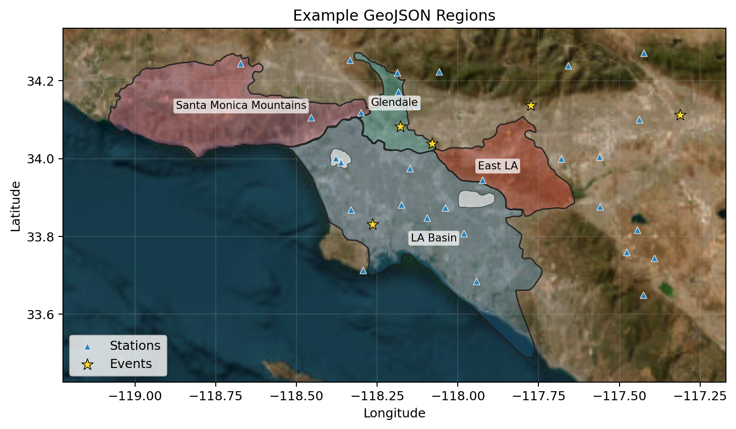
Run time: 14.35 s
Regional PGA Contrast
Add station-region labels from the GeoJSON file, then compare PGA residuals across stations that fall inside one of the example polygons. The table below the plot compares each mapped region against the LA Basin baseline.
[5]:
# Add station GeoJSON labels to each metric row.
metrics_by_station_region = add_geojson_metadata_to_metrics(
    metrics,
    geojson_path,
    target="station",
    selector="all",
)
metrics_by_station_region["station_region"] = metrics_by_station_region["station_geojson_labels"].str.replace("_", " ")

# Keep only stations that are inside one of the example polygons.
metrics_in_mapped_station_regions = metrics_by_station_region.loc[
    metrics_by_station_region["station_geojson_inside_any"].fillna(False)
    & metrics_by_station_region["station_geojson_labels"].astype(str).ne("")
].copy()

# Build a regional contrast boxplot for PGA residuals by station polygon.
pga_region_boxplot = boxplot(
    data=metrics_in_mapped_station_regions,
    dep="PGA",
    indep="station_region",
    value_col=value_column,
    passband=passbands,
    model=model_name,
    component=component,
    compare_to="LA Basin",
    table=True,
    title="PGA Residuals by Station Region",
    showfig=False,
    savefig=True,
    outpath=figure_dir / "step_05_pga_region_boxplot.png",
)
display(pga_region_boxplot)
plt.close(pga_region_boxplot)
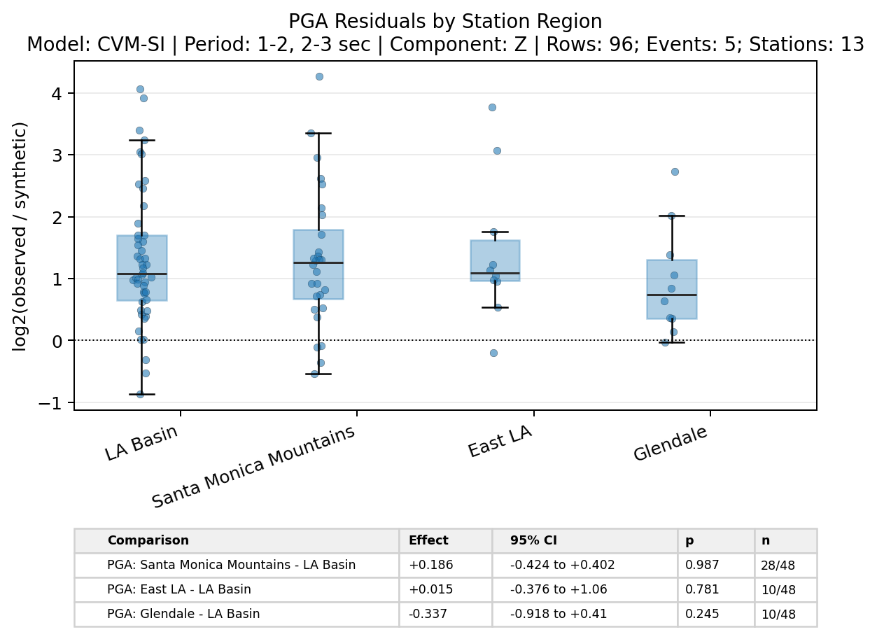
Run time: 1.18 s
Residual Map for Events and Stations in Different Regions
Here you can ask a more targeted question: for events in one polygon and stations in another, where are the average station residuals high or low? This example uses Glendale events recorded by LA Basin stations.
[6]:
# Add event-region labels to the same metric table.
metrics_by_regions = add_geojson_metadata_to_metrics(
    metrics_by_station_region,
    geojson_path,
    target="event",
    selector="all",
)
metrics_by_regions["event_region"] = metrics_by_regions["event_geojson_labels"].str.replace("_", " ")

# Keep PGA rows for Glendale events recorded at LA Basin stations.
regional_pga = metrics_by_regions.loc[
    metrics_by_regions["metric"].astype(str).eq("PGA")
    & metrics_by_regions["band"].astype(str).isin(passbands)
    & metrics_by_regions["component"].astype(str).eq(component)
    & metrics_by_regions["event_geojson_labels"].astype(str).eq(event_region)
    & metrics_by_regions["station_geojson_labels"].astype(str).eq(station_region)
].copy()

# Build a PGA residual field for that region-to-region subset.
regional_pga_field = build_metric_field(
    regional_pga,
    "PGA",
    value_column=value_column,
)

# Summarize mean station residuals without removing the event mean.
regional_pga_bias = summarize_station_bias(
    regional_pga_field,
    value_col="field_value",
    center_by_event=False,
    min_events_per_station=1,
)

# Keep the Glendale events visible behind the station residual markers.
regional_event_points = events.loc[events["event_id"].astype(str).isin(sorted(regional_pga["event_id"].astype(str).unique()))].copy()

# Map the station-mean PGA residuals with the Glendale and LA Basin polygons as faint context.
regional_pga_map = plot_station_metric_map(
    regional_pga_bias,
    value_col="mean_centered",
    lon_col="lon",
    lat_col="lat",
    events_df=regional_event_points,
    geojson_path=geojson_path,
    polygon_selector=[event_region, station_region],
    polygon_alpha=0.12,
    label_polygons=True,
    event_alpha=0.76,
    title="Mean PGA log2(obs/syn) Residual\nEvents in Glendale; Stations in LA Basin",
    showfig=False,
    savefig=True,
    outpath=figure_dir / "step_05_pga_glendale_events_la_basin_stations.png",
)
display(regional_pga_map)
plt.close(regional_pga_map)
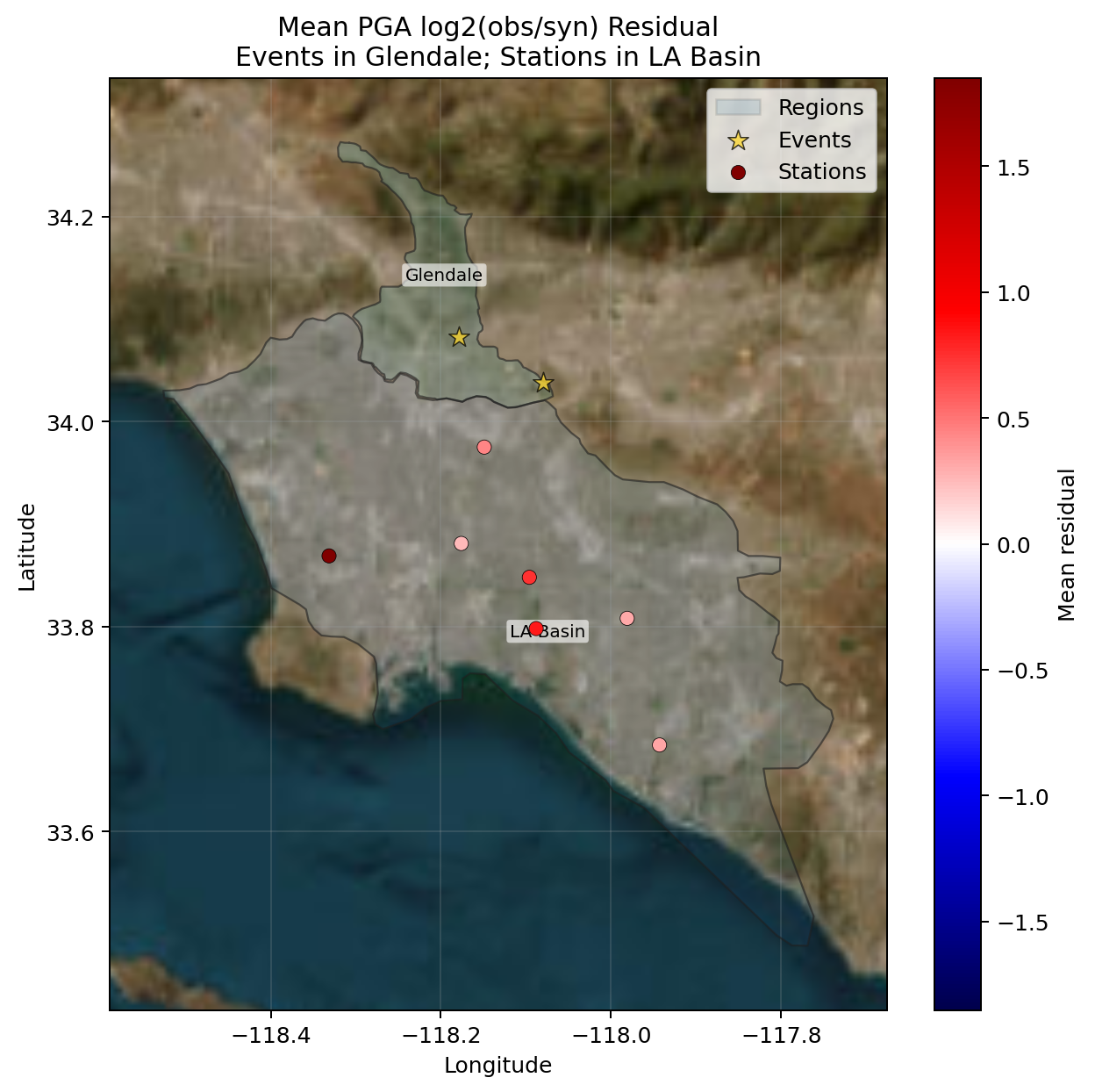
Run time: 2.08 s
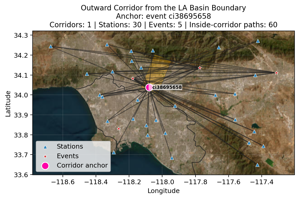
Define and Visualize Corridors
Corridors describe the part of a polygon boundary or near-boundary area you want to study. The examples below show two common options: a corridor crossing a boundary and a corridor going outward from a boundary.
[7]:
# Build a narrow corridor that extends both inside and outside the LA Basin boundary near station OLI.
through_corridors = build_boundary_corridors(
    geojson_path,
    config=BoundaryCorridorConfig(
        selector=boundary_region,
        mode="through_boundary",
        along_boundary_width_km=10,
        inside_length_km=15,
        outside_length_km=20,
        anchor=CorridorAnchorConfig(source="station", strategy="id", id_value=through_anchor_station),
    ),
    station_df=stations,
    event_df=events,
)

# Build a narrow corridor that starts at the LA Basin boundary and goes outward toward event ci38695658.
outward_corridors = build_boundary_corridors(
    geojson_path,
    config=BoundaryCorridorConfig(
        selector=boundary_region,
        mode="outward",
        along_boundary_width_km=10,
        inside_length_km=15,
        outside_length_km=20,
        anchor=CorridorAnchorConfig(source="event", strategy="id", id_value=outward_event_id),
    ),
    station_df=stations,
    event_df=events,
)

# Select paths that pass through the through-boundary corridor.
through_corridor_paths = select_records_by_corridors(
    event_stations,
    through_corridors,
    config=CorridorSelectionConfig(path_filter="passes_through_corridor", min_path_length_km=0.1),
)

# Select paths that pass through the outward corridor.
outward_corridor_paths = select_records_by_corridors(
    event_stations,
    outward_corridors,
    config=CorridorSelectionConfig(path_filter="passes_through_corridor", min_path_length_km=0.1),
)

# Plot the through-boundary corridor with matching event-station paths and the OLI anchor highlighted.
through_corridor_fig = plot_corridor_map(
    through_corridors,
    stations_df=stations,
    events_df=events,
    records_df=through_corridor_paths.drop_duplicates(["event_id", "station"]),
    highlight_anchor=True,
    title="Through-Boundary Corridor at the LA Basin Edge\nAnchor: station OLI",
    showfig=False,
    savefig=True,
    outpath=figure_dir / "step_05_corridor_through_boundary.png",
)
display(through_corridor_fig)
plt.close(through_corridor_fig)

# Plot the outward corridor with the paths that pass through its footprint and the event anchor highlighted.
outward_corridor_fig = plot_corridor_map(
    outward_corridors,
    stations_df=stations,
    events_df=events,
    records_df=outward_corridor_paths.drop_duplicates(["event_id", "station"]),
    highlight_anchor=True,
    title="Outward Corridor from the LA Basin Boundary\nAnchor: event ci38695658",
    showfig=False,
    savefig=True,
    outpath=figure_dir / "step_05_corridor_outward.png",
)
display(outward_corridor_fig)
plt.close(outward_corridor_fig)
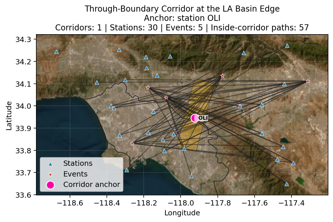
Run time: 2.85 s
Record Sections for Boundary-Crossing Paths
Now combine the polygon crossing test with the corridor selection. This cell keeps paths that cross the LA Basin boundary within the through-boundary corridor, then loads the QC-passed observed and synthetic waveforms for those paths.
[8]:
# Classify paths by whether they cross the LA Basin polygon boundary.
central_boundary_paths = classify_paths_with_geojson(
    event_stations,
    geojson_path,
    relation="crosses_boundary",
    selector=boundary_region,
    direction="either",
)

# Keep only paths that cross the boundary and pass through the through-boundary corridor.
boundary_crossing_paths = select_records_by_corridors(
    central_boundary_paths.loc[central_boundary_paths["path_geojson_matches"]].copy(),
    through_corridors,
    config=CorridorSelectionConfig(path_filter="passes_through_corridor", min_path_length_km=0.1),
)
selected_pairs = boundary_crossing_paths[["event_id", "station"]].drop_duplicates()
selected_eligible = comparison_eligible.merge(selected_pairs, on=["event_id", "station"], how="inner")

# Load QC-passed R-component observed/synthetic waveform pairs for the selected boundary-crossing paths.
boundary_waveforms = build_qc_waveform_comparison_records(
    event_stations,
    comparison_eligible=selected_eligible,
    component="R",
    passband="1-2 sec",
    max_distance_km=None,
    max_records=12,
)

# Plot the observed and synthetic records for the selected boundary-crossing paths.
boundary_record_section = plot_observed_synthetic_record_section(
    boundary_waveforms,
    components=["R"],
    normalize=True,
    scale=2.5,
    title="Observed vs Synthetic Records for LA Basin Boundary-Crossing Paths",
    filter_label="lowpass 1 Hz; R component; 1-2 sec QC passband",
    time_limit_s=60,
    showfig=False,
    savefig=True,
    outpath=figure_dir / "step_05_boundary_crossing_record_section.png",
)
display(boundary_record_section)
plt.close(boundary_record_section)

# Show the first few selected paths used by the record section.
boundary_crossing_paths[["event_id", "station", "distance_km", "path_length_in_corridor_km"]].drop_duplicates().head()
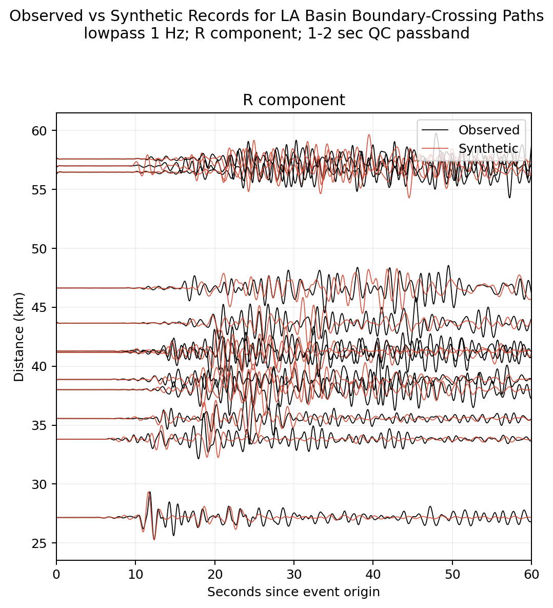
[8]:
| event_id | station | distance_km | path_length_in_corridor_km | |
|---|---|---|---|---|
| 0 | ci38038071 | BHP | 56.464515 | 5.657800 |
| 1 | ci38038071 | BRE | 41.169607 | 27.716130 |
| 2 | ci38038071 | CRF | 38.007905 | 23.725847 |
| 3 | ci38038071 | DLA | 43.652579 | 21.446123 |
| 4 | ci38038071 | FMP | 67.185917 | 19.614014 |
Run time: 4.24 s
PGV Residual Map for an Outward Corridor
Finally, select events inside the outward corridor and stations inside the LA Basin polygon. The map shows the station-mean PGV residuals for that corridor-based subset.
[9]:
# Select event-station rows whose events fall inside the outward corridor.
outward_event_paths = select_records_by_corridors(
    event_stations,
    outward_corridors,
    config=CorridorSelectionConfig(event_filter="inside_corridor"),
)
outward_event_ids = sorted(outward_event_paths["event_id"].dropna().astype(str).unique())
events_in_outward_corridor = events.loc[events["event_id"].astype(str).isin(outward_event_ids)].copy()
selected_event_names = events_in_outward_corridor[["event_id", "event_name"]].drop_duplicates()

display(Markdown("### Events inside the outward corridor"))
display(selected_event_names)

# Keep PGV rows for events inside the outward corridor and stations inside the LA Basin polygon.
pgv_corridor_rows = metrics_by_regions.loc[
    metrics_by_regions["metric"].astype(str).eq("PGV")
    & metrics_by_regions["band"].astype(str).isin(passbands)
    & metrics_by_regions["component"].astype(str).eq(component)
    & metrics_by_regions["event_id"].astype(str).isin(outward_event_ids)
    & metrics_by_regions["station_geojson_labels"].astype(str).eq(corridor_station_region)
].copy()

# Build a PGV residual field for the corridor-selected subset.
pgv_corridor_field = build_metric_field(
    pgv_corridor_rows,
    "PGV",
    value_column=value_column,
)

# Summarize mean station residuals without removing the event mean.
pgv_corridor_bias = summarize_station_bias(
    pgv_corridor_field,
    value_col="field_value",
    center_by_event=False,
    min_events_per_station=1,
)

# Keep the plotted event-station paths for the same events and LA Basin stations shown on the residual map.
pgv_corridor_pairs = pgv_corridor_rows[["event_id", "station"]].drop_duplicates()
pgv_corridor_paths = outward_event_paths.merge(pgv_corridor_pairs, on=["event_id", "station"], how="inner")

# Map station-mean PGV residuals with the outward corridor, selected events, and selected paths overlaid.
pgv_corridor_map = plot_station_metric_map(
    pgv_corridor_bias,
    value_col="mean_centered",
    lon_col="lon",
    lat_col="lat",
    geojson_path=geojson_path,
    polygon_selector="all",
    polygon_alpha=0.10,
    label_polygons=True,
    corridors_df=outward_corridors,
    events_df=events_in_outward_corridor,
    records_df=pgv_corridor_paths.drop_duplicates(["event_id", "station"]),
    title="Mean PGV log2(obs/syn) Residual\nEvents in Outward Corridor; Stations in LA Basin",
    showfig=False,
    savefig=True,
    outpath=figure_dir / "step_05_pgv_outward_corridor_la_basin_stations.png",
)
display(pgv_corridor_map)
plt.close(pgv_corridor_map)
Events inside the outward corridor
| event_id | event_name | |
|---|---|---|
| 1 | ci38695658 | M 4.5 - 3km WSW of South El Monte, CA |
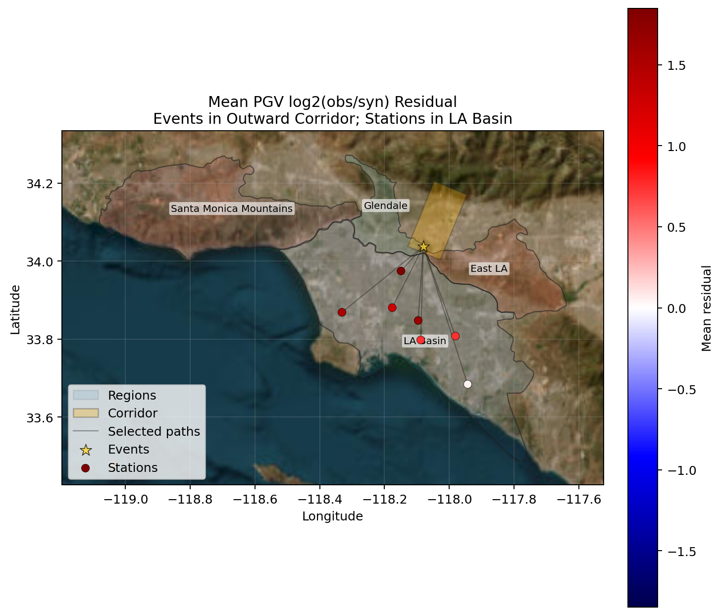
Run time: 2.01 s