Download this notebook

Step 4: Add Metadata and Analyze Spatial Patterns

This notebook turns metric results into spatial summaries. You will use PGA and FAS as two separate examples, so you can see how the same spatial tests can highlight different model-performance patterns for different metrics.

Imports

These functions prepare metric fields and calculate spatial summaries.

from spatial_vtk.config.notebook import notebook_timer, register_svtk_cell_timer

with notebook_timer():
    import os

    os.environ.setdefault("LOKY_MAX_CPU_COUNT", "1")

    from pathlib import Path
    import pandas as pd
    from IPython.display import Markdown, display

    from spatial_vtk.config import SpatialVTKConfig
    from spatial_vtk.config.labels import metric_display_name
    from spatial_vtk.io import read_config_table, write_output_tables
    from spatial_vtk.spatial.calculate import (
        bootstrap_contrast_table,
        build_distance_bin_summary,
        build_metric_field,
        build_station_feature_table,
        center_field_by_event,
        compute_global_morans_i,
        compute_pca_spatial_modes,
        moran_result_to_frame,
        normalize_metrics_table,
        run_residual_feature_clustering,
        summarize_station_bias,
    )
    from spatial_vtk.spatial.map import plot_residual_grid, plot_station_bias_map
    from spatial_vtk.spatial.map.pca import plot_pca_summary
    from spatial_vtk.spatial.plot import plot_distance_correlation_by_metric, plot_geology_contrast
    register_svtk_cell_timer()

Run time: 4.00 s

Configuration

Load the config and read the spatial-statistics settings from the tutorial run scenario.

# Use the repository root so paths match the public source checkout.
repo_root = Path.cwd()
config_path = repo_root / "data/examples/configuration/example_spatial_vtk_config.yaml"

# Load the tutorial run scenario and make it the active config for later package calls.
cfg = SpatialVTKConfig.from_file(config_path, run_scenario="tutorial").activate()

# Step 4 uses a larger QC-passed metrics snapshot so per-metric spatial tests have enough stations.
metric_source_path = cfg.path("paths.metric_figure_snapshot")
figure_dir = cfg.path("outputs.figures")
figure_dir.mkdir(parents=True, exist_ok=True)
spatial_metrics = ("PGA", "FAS")
spatial_value_column = "log2_residual"

Run time: 23.2 ms

Prepare Metric-Specific Spatial Fields

Spatial statistics use one value per event-station observation, plus station and event coordinates. Here you will build those fields separately for PGA and FAS. The tutorial snapshot has broader station coverage for PGA than FAS after QC, so the FAS examples will use fewer stations.

# Read the larger QC-passed metric snapshot used for spatial tutorial examples.
metrics = pd.read_parquet(metric_source_path)

# Read the configured site/geology metadata table.
site_metadata = read_config_table("paths.site_metadata")

# Normalize metric columns so spatial-statistics helpers see consistent names.
spatial_ready = normalize_metrics_table(metrics)

spatial_products = {}
for metric_name in spatial_metrics:
    display(Markdown(f"### {metric_display_name(metric_name)}"))

    # Build one event-station field for this metric using log2(observed/synthetic) residuals.
    field = build_metric_field(spatial_ready, metric=metric_name, value_column=spatial_value_column)

    # Remove each event mean before comparing persistent station patterns.
    centered = center_field_by_event(field)

    # Summarize each station's mean event-centered residual for this metric.
    station_bias = summarize_station_bias(centered)

    spatial_products[metric_name] = {
        "field": field,
        "centered": centered,
        "station_bias": station_bias,
    }

    display(
        pd.DataFrame(
            {
                "Output": ["Metric field", "Event-centered field", "Station bias"],
                "Rows": [len(field), len(centered), len(station_bias)],
                "Events": [field["event_id"].nunique(), centered["event_id"].nunique(), ""],
                "Stations": [field["station"].nunique(), centered["station"].nunique(), station_bias["station"].nunique()],
            }
        )
    )
    display(station_bias.head())

metric_field = pd.concat([item["field"] for item in spatial_products.values()], ignore_index=True)
event_centered_residuals = pd.concat([item["centered"] for item in spatial_products.values()], ignore_index=True)
station_bias = pd.concat([item["station_bias"].assign(metric=metric_name) for metric_name, item in spatial_products.items()], ignore_index=True)

# Save the core spatial-statistics handoff tables for later notebooks.
write_output_tables(
    metric_field=metric_field,
    event_centered_residuals=event_centered_residuals,
    station_bias=station_bias,
)

Peak acceleration (PGA)

	Output	Rows	Events	Stations
0	Metric field	190	5	27
1	Event-centered field	190	5	27
2	Station bias	27		27

	station	lat	lon	n_events	mean_centered	median_centered	std_centered	sem_centered	abs_mean_centered	bias_zscore
15	LAF	33.86889	-118.33143	4	0.766314	0.656147	0.773329	0.386664	0.766314	1.981858
20	LMH	33.74400	-117.39100	3	-0.726876	-0.791837	0.434740	0.250997	0.726876	-2.895954
21	LMS	33.81700	-117.44500	3	-0.678520	-0.560183	1.070426	0.618011	0.678520	-1.097910
10	ELS2	33.64907	-117.42604	4	-0.675554	-0.647399	0.780660	0.390330	0.675554	-1.730725
8	DJJ	34.10618	-118.45505	5	-0.582270	-0.582530	0.685731	0.306668	0.582270	-1.898697

Fourier amplitude spectrum (FAS)

	Output	Rows	Events	Stations
0	Metric field	62	5	7
1	Event-centered field	62	5	7
2	Station bias	7		7

	station	lat	lon	n_events	mean_centered	median_centered	std_centered	sem_centered	abs_mean_centered	bias_zscore
3	BRE	33.808	-117.981	3	-0.665123	-0.597910	1.268973	0.732642	0.665123	-0.907842
0	BFS	34.239	-117.659	4	-0.600799	-0.664543	1.218519	0.609260	0.600799	-0.986113
2	BLC	34.244	-118.673	4	0.522485	0.882365	1.305393	0.652697	0.522485	0.800502
4	CHN	33.999	-117.680	3	0.473351	0.143310	1.354242	0.781872	0.473351	0.605407
5	CJM	34.271	-117.424	3	0.224016	0.446772	0.708175	0.408865	0.224016	0.547898

{'metric_field': PosixPath('outputs/tutorials/tables/metric_field.parquet'),
 'event_centered_residuals': PosixPath('outputs/tutorials/tables/event_centered_residuals.parquet'),
 'station_bias': PosixPath('outputs/tutorials/tables/station_bias.parquet')}

Run time: 6.53 s

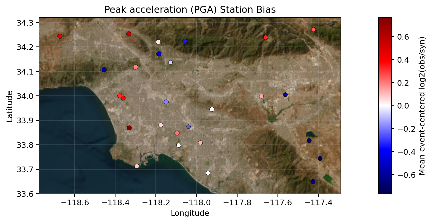
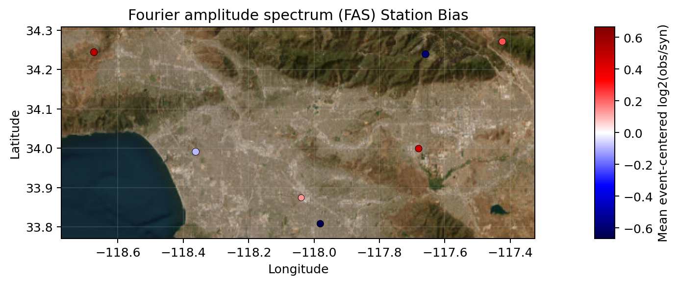
Station Bias Maps

These maps show the mean event-centered residual at each station. Positive values mean the observed amplitudes are larger than the synthetic amplitudes on average for that metric.

for metric_name, products in spatial_products.items():
    display(Markdown(f"### {metric_display_name(metric_name)}"))

    # Map the mean event-centered residual at each station for this metric.
    station_bias_fig = plot_station_bias_map(
        products["station_bias"],
        title=f"{metric_display_name(metric_name)} Station Bias",
        value_col="mean_centered",
        value_label="Mean event-centered log2(obs/syn)",
        add_basemap=True,
        showfig=True,
        savefig=True,
        outpath=figure_dir / f"step_04_{metric_name.lower()}_station_bias.png",
    )

Peak acceleration (PGA)

Fourier amplitude spectrum (FAS)

Run time: 16.16 s

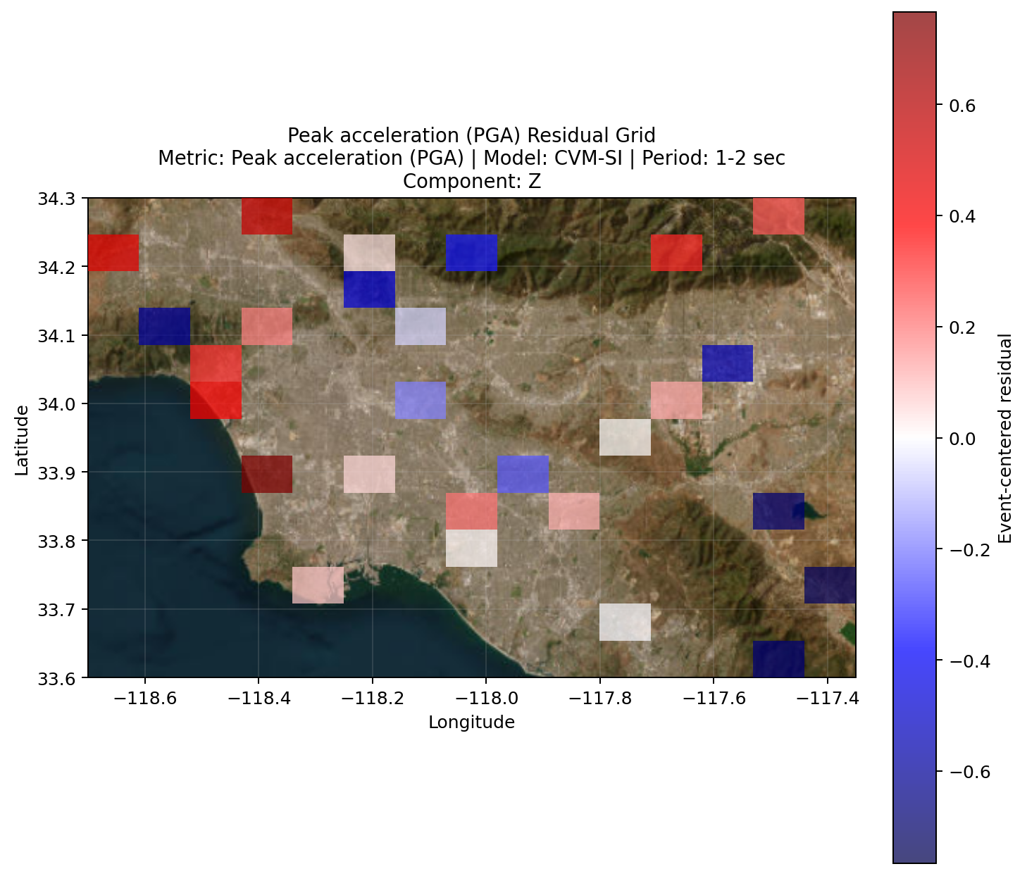
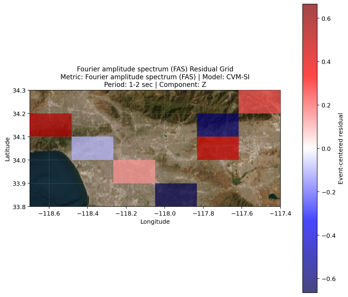
Residual Grid Maps

A residual grid gives you a quick spatial overview of where residuals are broadly positive or negative. These examples use the same event-centered residual field as the station-bias maps.

for metric_name, products in spatial_products.items():
    display(Markdown(f"### {metric_display_name(metric_name)}"))

    # Grid event-centered residuals onto lon/lat cells for a broader spatial view.
    residual_grid_fig = plot_residual_grid(
        products["centered"],
        lon_col="lon",
        lat_col="lat",
        value_col="field_centered",
        cell_size_deg=0.05,
        title=f"{metric_display_name(metric_name)} Residual Grid",
        add_basemap=True,
        showfig=True,
        savefig=True,
        outpath=figure_dir / f"step_04_{metric_name.lower()}_residual_grid.png",
    )

Peak acceleration (PGA)

Fourier amplitude spectrum (FAS)

Run time: 3.24 s

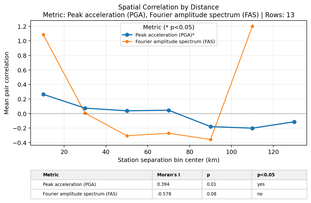
Spatial Correlation Tests

Moran’s I and distance-bin correlations help you see whether residuals cluster in space. Run them separately for each metric so the results are easier to interpret, then plot the distance-binned correlations together to compare the spatial pattern.

moran_tables = {}
distance_bin_tables = {}

for metric_name, products in spatial_products.items():
    display(Markdown(f"### {metric_display_name(metric_name)}"))

    # Compute global Moran's I for this metric's station-bias field.
    moran_result = compute_global_morans_i(products["station_bias"])

    # Convert the Moran result object into a table for saving and display.
    morans_i = moran_result_to_frame(moran_result).assign(metric=metric_name)

    # Summarize residual similarity as a function of station separation distance for this metric.
    distance_bins = build_distance_bin_summary(products["centered"]).assign(metric=metric_name)

    moran_tables[metric_name] = morans_i
    distance_bin_tables[metric_name] = distance_bins
    display(morans_i)
    display(distance_bins.head())

morans_i = pd.concat(moran_tables.values(), ignore_index=True)
distance_bins = pd.concat(distance_bin_tables.values(), ignore_index=True)

# Plot correlation as a function of station separation distance for the selected metrics.
correlation_distance_fig = plot_distance_correlation_by_metric(
    distance_bins,
    significance_df=morans_i,
    title="Spatial Correlation by Distance",
    showfig=True,
    savefig=True,
    outpath=figure_dir / "step_04_spatial_correlation_distance.png",
)

# Save the spatial-correlation result tables.
write_output_tables(
    morans_i=morans_i,
    permutation_moran=morans_i,
    distance_bin_correlations=distance_bins,
)

Peak acceleration (PGA)

	n	k	moran_i	p_two_sided	permutations	metric
0	27	2	0.393745	0.01	99	PGA

	distance_start_km	distance_end_km	distance_center_km	pair_count	event_count	mean_pair_correlation	mean_semivariance	metric
0	0.0	20.0	10.0	125	5	0.264176	0.506715	PGA
1	20.0	40.0	30.0	260	5	0.074086	0.513820	PGA
2	40.0	60.0	50.0	232	5	0.037790	0.509227	PGA
3	60.0	80.0	70.0	142	5	0.045500	0.535277	PGA
4	80.0	100.0	90.0	98	5	-0.179900	0.853431	PGA

Fourier amplitude spectrum (FAS)

	n	k	moran_i	p_two_sided	permutations	metric
0	7	2	-0.577606	0.08	99	FAS

	distance_start_km	distance_end_km	distance_center_km	pair_count	event_count	mean_pair_correlation	mean_semivariance	metric
0	0.0	20.0	10.0	1	1	1.086162	0.159007	FAS
1	20.0	40.0	30.0	12	4	0.005452	0.835103	FAS
2	40.0	60.0	50.0	10	3	-0.304875	2.273905	FAS
3	60.0	80.0	70.0	8	3	-0.271107	1.470696	FAS
4	80.0	100.0	90.0	10	3	-0.356686	2.729818	FAS

{'morans_i': PosixPath('outputs/tutorials/tables/morans_i.csv'),
 'permutation_moran': PosixPath('outputs/tutorials/tables/permutation_moran.csv'),
 'distance_bin_correlations': PosixPath('outputs/tutorials/tables/distance_bin_correlations.csv')}

Run time: 676.0 ms

Clustering and PCA Spatial Modes

These summaries group stations with similar residual fingerprints and identify dominant station-level patterns. You will create a PCA summary figure for PGA and another one for FAS.

cluster_tables = []
cluster_score_tables = []
cluster_summary_tables = []
pca_score_tables = []
pca_loading_tables = []
pca_variance_tables = []

for metric_name, products in spatial_products.items():
    display(Markdown(f"### {metric_display_name(metric_name)}"))

    # Build a station-by-event residual matrix for this metric.
    feature_table = build_station_feature_table(products["centered"])

    # Cluster stations with similar event-centered residual patterns for this metric.
    cluster_assignments, cluster_scores, cluster_features, cluster_summary, best_cluster, cluster_feature_columns = run_residual_feature_clustering(feature_table)

    # Decompose this metric's station residual patterns into PCA spatial modes.
    pca_result = compute_pca_spatial_modes(feature_table)

    # Plot the PC1 map, explained variance, and feature loading summary for this metric.
    pca_summary_fig = plot_pca_summary(
        pca_result.station_scores,
        pca_result.explained_variance,
        pca_result.feature_loadings,
        mode="PC1",
        title=f"{metric_display_name(metric_name)} PCA Spatial Mode Summary",
        add_basemap=True,
        showfig=True,
        savefig=True,
        outpath=figure_dir / f"step_04_{metric_name.lower()}_pca_summary.png",
    )

    cluster_tables.append(cluster_assignments.assign(metric=metric_name))
    cluster_score_tables.append(cluster_scores.assign(metric=metric_name))
    cluster_summary_tables.append(cluster_summary.assign(metric=metric_name))
    pca_score_tables.append(pca_result.station_scores.assign(metric=metric_name))
    pca_loading_tables.append(pca_result.feature_loadings.assign(metric=metric_name))
    pca_variance_tables.append(pca_result.explained_variance.assign(metric=metric_name))
    display(pca_result.explained_variance)

clusters = pd.concat(cluster_tables, ignore_index=True)
cluster_scores = pd.concat(cluster_score_tables, ignore_index=True)
cluster_summary = pd.concat(cluster_summary_tables, ignore_index=True)
pca_station_scores = pd.concat(pca_score_tables, ignore_index=True)
pca_feature_loadings = pd.concat(pca_loading_tables, ignore_index=True)
pca_explained_variance = pd.concat(pca_variance_tables, ignore_index=True)

# Save clustering and PCA tables for the mapping notebook.
write_output_tables(
    clusters=clusters,
    cluster_scores=cluster_scores,
    cluster_summary=cluster_summary,
    pca_station_scores=pca_station_scores,
    pca_feature_loadings=pca_feature_loadings,
    pca_explained_variance=pca_explained_variance,
)

Peak acceleration (PGA)

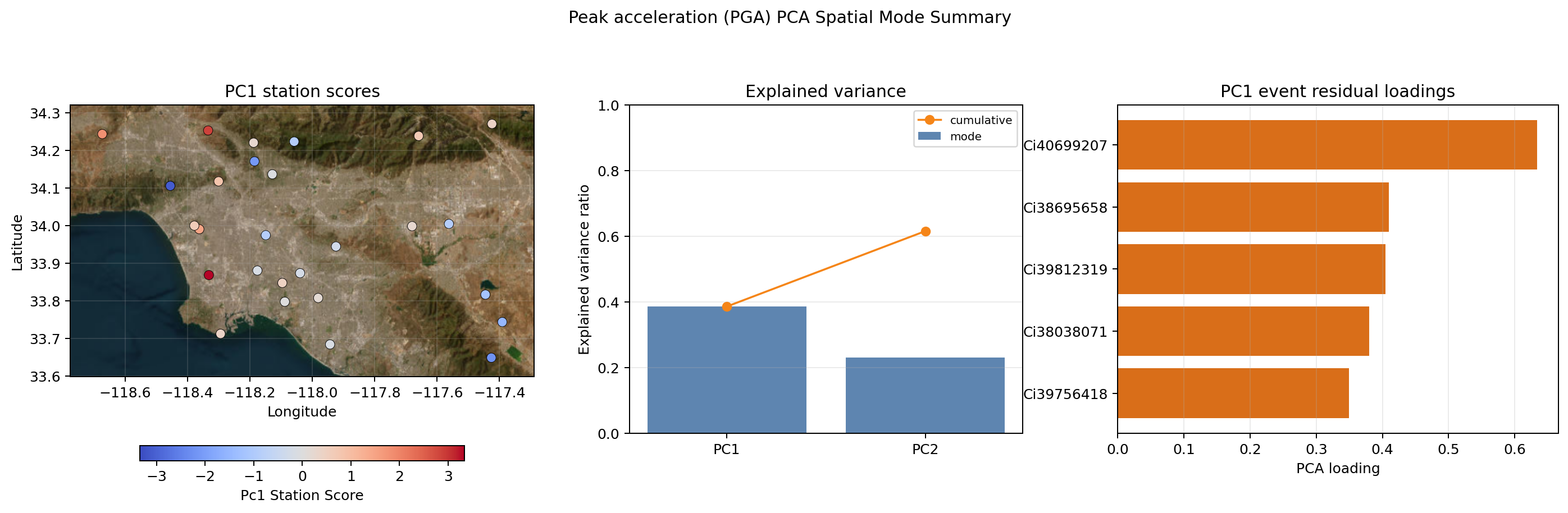
	mode	mode_index	explained_variance	explained_variance_ratio	cumulative_explained_variance_ratio	singular_value	n_stations	n_features	standardized
0	PC1	1	2.003519	0.385863	0.385863	7.217443	27	5	True
1	PC2	2	1.194923	0.230133	0.615996	5.573868	27	5	True

Fourier amplitude spectrum (FAS)

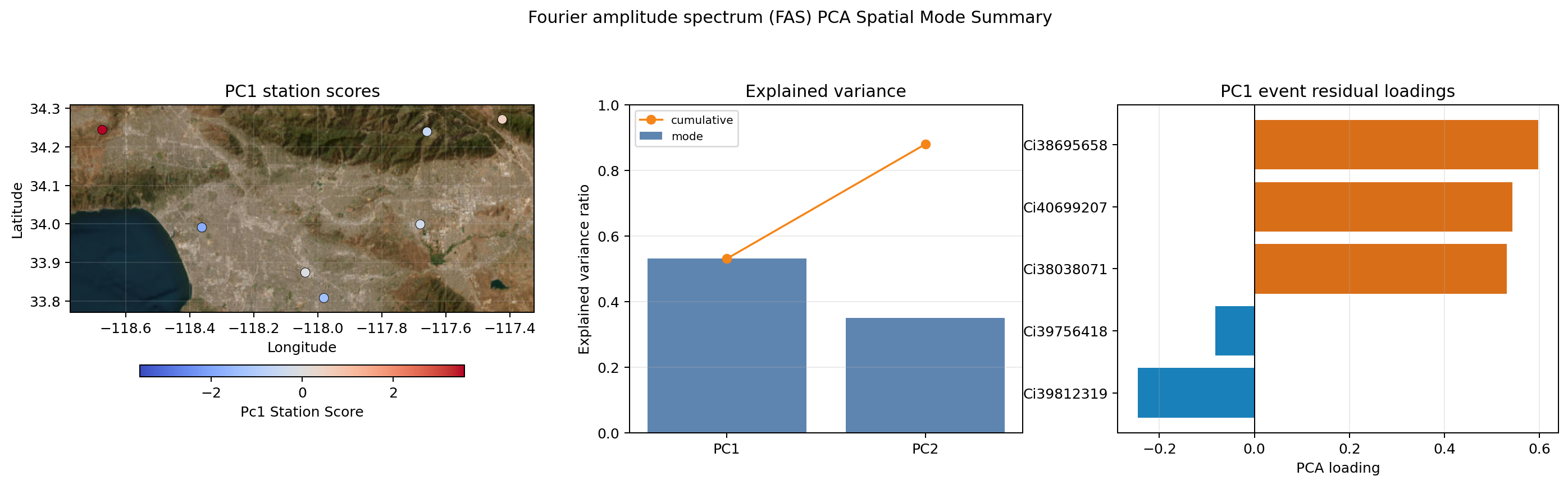
	mode	mode_index	explained_variance	explained_variance_ratio	cumulative_explained_variance_ratio	singular_value	n_stations	n_features	standardized
0	PC1	1	3.096483	0.530826	0.530826	4.310325	7	5	True
1	PC2	2	2.040406	0.349784	0.880609	3.498919	7	5	True

{'clusters': PosixPath('outputs/tutorials/tables/clusters.parquet'),
 'cluster_scores': PosixPath('outputs/tutorials/tables/cluster_scores.csv'),
 'cluster_summary': PosixPath('outputs/tutorials/tables/cluster_summary.csv'),
 'pca_station_scores': PosixPath('outputs/tutorials/tables/pca_station_scores.parquet'),
 'pca_feature_loadings': PosixPath('outputs/tutorials/tables/pca_feature_loadings.csv'),
 'pca_explained_variance': PosixPath('outputs/tutorials/tables/pca_explained_variance.csv')}

Run time: 3.32 s

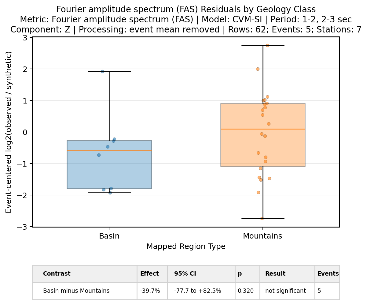
Geology Contrasts

Compare PGA and FAS residuals across the configured geology classes. GeoJSON regions and corridors are handled in the next notebook.

geology_tables = []

for metric_name, products in spatial_products.items():
    display(Markdown(f"### {metric_display_name(metric_name)}"))

    # Compare configured geology classes with an event-bootstrap uncertainty estimate for this metric.
    geology_contrast = bootstrap_contrast_table(products["centered"], station_metadata=site_metadata).assign(metric=metric_name)

    # Plot the residual distributions and annotate the configured geology-class contrast for this metric.
    geology_contrast_fig = plot_geology_contrast(
        products["centered"],
        station_metadata=site_metadata,
        contrast_df=geology_contrast,
        title=f"{metric_display_name(metric_name)} Residuals by Geology Class",
        showfig=True,
        savefig=True,
        outpath=figure_dir / f"step_04_{metric_name.lower()}_geology_contrast.png",
    )

    geology_tables.append(geology_contrast)
    display(geology_contrast)

geology_contrasts = pd.concat(geology_tables, ignore_index=True)

# Save the geology contrast output for later review.
write_output_tables(geology_contrasts=geology_contrasts)

Peak acceleration (PGA)

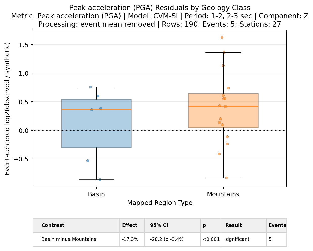
	group_col	left_values	right_values	comparison_values	baseline_values	contrast_label	effect_direction	value_col	statistic	min_stations_per_group	...	bootstrap_p	significant_95	significant_p05	n_left_stations	n_right_stations	n_comparison_stations	n_baseline_stations	n_events	bootstrap_samples_used	metric
0	mapped_region_type	Basin	Mountains	Basin	Mountains	Basin minus Mountains	mean(Basin) - mean(Mountains)	field_centered	mean	1	...	0.0	True	True	1	2	1	2	5	100	PGA

1 rows × 26 columns

Fourier amplitude spectrum (FAS)

	group_col	left_values	right_values	comparison_values	baseline_values	contrast_label	effect_direction	value_col	statistic	min_stations_per_group	...	bootstrap_p	significant_95	significant_p05	n_left_stations	n_right_stations	n_comparison_stations	n_baseline_stations	n_events	bootstrap_samples_used	metric
0	mapped_region_type	Basin	Mountains	Basin	Mountains	Basin minus Mountains	mean(Basin) - mean(Mountains)	field_centered	mean	1	...	0.32	False	False	1	2	1	2	5	100	FAS

1 rows × 26 columns

{'geology_contrasts': PosixPath('outputs/tutorials/tables/geology_contrasts.csv')}

Run time: 1.01 s